In
the previous couple of posts I discussed the application of both regression
(estimation of a continuous output for a given input sample) and
classification (estimation of the class to which a given input sample
belongs) machine learning methods with application to socio-economic
data. Specifically multi-dimensional linear regression was used to
estimate the average life expectancy for a particular country from a
series of continuous socio-economic factors. Logistic regression was
also used to classify if a country belonged to the OECD or not in a
particular year. Here I will illustrate a way
to build predictive classification models using artificial
neural networks
(ANN) machine learning algorithms.
The formulation of ANNs is inspired by the structure of the brain. They are represented as a network of interconnected neurons, and are used to learn both regression and classification functions from data samples comprising of potentially a large number of input variables. This general approach has produced state-of-the-art results in computer vision, speech recognition and natural language processing [1,2,3]. ANNs are also referred to as feed-forward neural network, multi-layer perception, and more recently deep networks/learning. Deep learning has come to represent applications in which the amount of feature engineering is minimised, with the machine learning tasks achieved through multiple learned layers of neurons. Each neuron undertakes a weighted sum over a series of inputs then applies a nonlinear activation function producing an output value, as illustrated below. For regression problems the rectified linear unit (ReLU) is a popular activation function. For classification problems the sigmoid or hyperbolic tangent functions as used in logistic regression are the most common activations functions.
The formulation of ANNs is inspired by the structure of the brain. They are represented as a network of interconnected neurons, and are used to learn both regression and classification functions from data samples comprising of potentially a large number of input variables. This general approach has produced state-of-the-art results in computer vision, speech recognition and natural language processing [1,2,3]. ANNs are also referred to as feed-forward neural network, multi-layer perception, and more recently deep networks/learning. Deep learning has come to represent applications in which the amount of feature engineering is minimised, with the machine learning tasks achieved through multiple learned layers of neurons. Each neuron undertakes a weighted sum over a series of inputs then applies a nonlinear activation function producing an output value, as illustrated below. For regression problems the rectified linear unit (ReLU) is a popular activation function. For classification problems the sigmoid or hyperbolic tangent functions as used in logistic regression are the most common activations functions.

The input variables in a ANN are introduced into an input layer. These inputs are fed into a hidden layer of neurons. The outputs from the first hidden layer may then be fed into a second hidden layer. There may well be many hidden layers, with each layer learning more complex and more specialised behaviour. The penultimate hidden layer feeds its outputs to the final output layer. This typical structure of an ANN is illustrated below. Each circle represents a neuron, and the lines represent the interconnections. For a given network, the credit assignment path (CAP) is the path of nonlinear functions from an input to the output. The length of the CAP for a feed-forward neural network is the number of hidden layers plus one for the output layer. In recurrent neural networks a signal may pass through a given layer on multiple occasions, which means the length of the CAP is unbounded.

The weights in each neuron are learnt from the training data, such that they minimise a specified cost function. The cost function comprises of a loss (or error) function element that quantifies the difference between the value estimated by the ANN and the true value. For regression problems one would use a least squares error measure, whilst for classification problems a log-likelihood (or information entropy) measure is more appropriate. The cost function may also contain some additional regularisation terms which specify the relative importance put on minimising the amplitude of the model weights.
In ANNs the cost function
is typically minimised using the back-propagation method. In
the standard back-propagation method the weights are updated using
some form of convex optimisation method, such as the gradient decent algorithm. In the gradient decent algorithm one first calculates the gradient/derivative of (change in) the cost function with respect to the
weights, with the gradient averaged across all samples in the training set. The value of each weight from the previous iteration is then updated by adding to it the cost function gradient multiplied by a specified constant rate of learning. Here I adopt the mini-batch stochastic gradient descent variant, where the cost function gradient is averaged over only a small batch of samples in the training set, as opposed to all of the available samples. The larger the batch size the better the estimate of the gradient, but the more time taken to calculate the gradient. The batch size that returns the model coefficients with the least amount of computational resources is problem dependent, but typically ranges in order from 1 to 100 [4]. A very good explanation and illustration of the back-propagation method and gradient decent algorithm can be found in [5].
There
are various frameworks available for creating ANN applications
including:
- Theano is a python library developed at University of Montreal, which calculates the partial derivatives required for the back-propagation algorithm using symbolic mathematics [4,6,7].
- Torch is a deep learning framework developed using the Lua programming language, and is currently being co-developed and maintained by researchers at facebook, google deepmind, twitter and New York University.
- DeepLearning4J is an open-source, parallel deep-learning library for Java and Scala, which can be integrated with Hadoop and Spark databases management systems.
- Caffe is a C++ deep learning framework developed at Berkeley University with python and matlab interfaces.
As an illustration I have repeated the OECD classification problem solved in the previous blog post using logistic regression. To briefly recap the goal is to build a classification model determining if a particular country in a particular year is in the OECD on the basis of various socio-economic measures including: GDP; average life expectancy; average years spent in school; population growth; and money spent on health care amongst others. Here the classification problem is solved using a ANN with 12 input variables, one hidden layer comprising of 24 neurons, all of which feeding into one output neuron. A hyperbolic tangent activation function is used for the hidden layer neurons, and a sigmoid activation function for the output neuron. The model weights are randomly initialised using a uniform probability distribution. The code is written in python using the theano library.
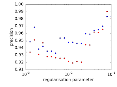
The ANN is calculated over the training data set using L2 regularisation, with the regularisation parameters ranging from 0.001 and 0.1. The predictive performance measures of precision (P = [True positive] / [True positive + False positive], recall (R = [True positive] / [True positive + False negative]) and F1 score (2P*R/(P+R)) are calculated for each regularisation parameter over the training and validation data sets and illustrated in the following figures. As expected each performance measure of is greater for training data set than the validation data set across most regularisation levels.


 One
final note, ANNs are biologically inspired learning algorithms, but
the mathematical form of the neurons is far simpler than the behaviour of biological neurons. There are a range of methods that aim to more
closely replicate the learning processes in the brain. The human
brain actually consists of several levels (of which neurons are only one),
each of which serve a slightly different purpose in the learning
process [8]. Algorithms that attempt to replicate this process are
refereed to as cortical learning algorithms.
One
final note, ANNs are biologically inspired learning algorithms, but
the mathematical form of the neurons is far simpler than the behaviour of biological neurons. There are a range of methods that aim to more
closely replicate the learning processes in the brain. The human
brain actually consists of several levels (of which neurons are only one),
each of which serve a slightly different purpose in the learning
process [8]. Algorithms that attempt to replicate this process are
refereed to as cortical learning algorithms.
The ANN is calculated over the training data set using L2 regularisation, with the regularisation parameters ranging from 0.001 and 0.1. The predictive performance measures of precision (P = [True positive] / [True positive + False positive], recall (R = [True positive] / [True positive + False negative]) and F1 score (2P*R/(P+R)) are calculated for each regularisation parameter over the training and validation data sets and illustrated in the following figures. As expected each performance measure of is greater for training data set than the validation data set across most regularisation levels.


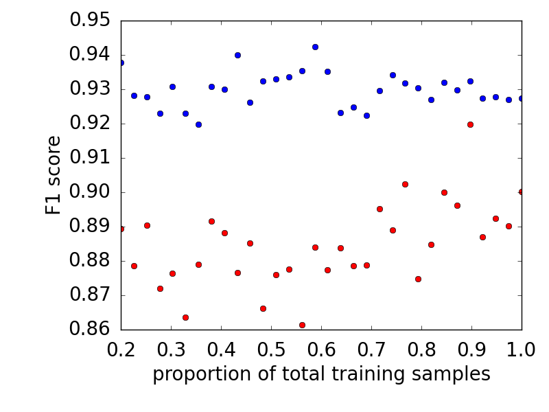
The ANN with the greatest F1 score over the validation data set has a regularisation level of 0.001. The learning curves illustrating the F1 curve as a function of the number of samples used to train this particular model is illustrated below. The fact that the learning curves of the training and validation data sets do not converge indicate that the predictive performance could be further improved with additional data.
References:
[1]
http://yann.lecun.com/exdb/mnist/
[2]
Deng, L.; Li, Xiao (2013). "Machine Learning Paradigms for
Speech Recognition: An Overview". IEEE Transactions on Audio,
Speech, and Language Processing.
[3]
Socher, Richard (2013). "Recursive Deep Models for Semantic
Compositionality Over a Sentiment Treebank"
[4] LISA lab (2015), "Deep Learning Tutorial", University of Montreal.
[4] LISA lab (2015), "Deep Learning Tutorial", University of Montreal.
[6]
F.
Bastien, P. Lamblin, R. Pascanu, J. Bergstra, I. Goodfellow, A.
Bergeron, N. Bouchard, D. Warde-Farley and Y. Bengio. “Theano:
new features and speed improvements”.
NIPS 2012 deep learning workshop.
[7]
J. Bergstra, O. Breuleux, F. Bastien, P. Lamblin, R. Pascanu, G.
Desjardins, J. Turian, D. Warde-Farley and Y. Bengio. “Theano:
A CPU and GPU Math Expression Compiler”. Proceedings
of the Python for Scientific Computing Conference (SciPy) 2010. June
30 - July 3, Austin, TX
[8]
https://www.youtube.com/watch?v=6ufPpZDmPKA